| Previous Page | Contents | Next Page |
The best way to learn how a program works is to use it, so let's do that. We'll reduce a run taken with a 2-channel photometer in 1989, as part of the WET run we call Xcov3. If a few things seem a bit mysterious in this quick run-through, don't worry. When you finish this document you'll know more than you wanted to know about Qed.
At the MS-DOS prompt, we type the command
qed raw\tol-0011
and, assuming the data file is in the directory raw\, we'll see this screen:
This is called the Set mode window, and there is a simple editor under the hood that will let you modify most of the entries if you need to, but mostly you won't. This image (in glorious black and white) is what you will see on the screen: white letters on a black background. For the Run mode images you'll see the same, but in this document they have been reversed so data points appear black, on a white background, to make individual points a bit easier to see. If you click on the links below, the colored ones just below the image, a new window will pop up to show you the same image, animated so you can see what is blinking. Dismiss it when you're finished: these are animated GIF images, and if you keep popping up new windows, you'll run out of CPU cycles very quickly.
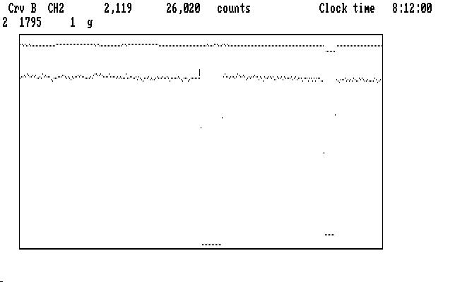
The Esc key switches the display to Run mode, shown below, so we can get to work:
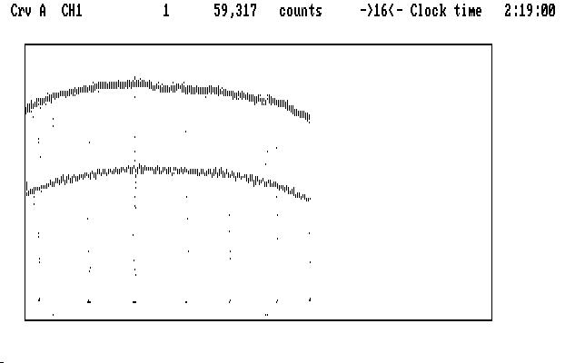
| Fig. T01 |
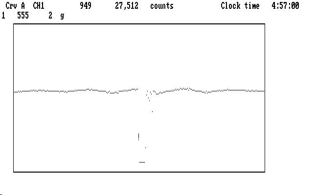
The top curve is Ch2, the monitor star, which should be flat; so should the lower curve, Ch1. They aren't, and there are a bunch of points that don't lie on either curve. Our job is to fix these things. As we do, the text on the top line will change, showing useful things about the display and the data point we have selected (with the cursor, the short vertical line above the leftmost datum on the Ch1 curve).
The display is compressed, so you can see the whole run at a glance, and we must uncompress it so we can deal with the individual data points. We'll start with Ch1, so use Alt-Del to make Ch2 go away, then press the Tab key (to move the cursor to the center of the screen; the curve will follow) and then 'x'. The display now looks like this:
| Fig. T02 |
The Left arrow key '<-' moves the curve to the left but the cursor stays put, so we can scan the data points past it and mark them. There are some low points we want to mark as garbage (put the cursor on one of them, then the 'g' key does that, and advances the curve one notch to the next data point).
The very low group of points, like a flat-bottomed eclipse, are sky measurements and should be marked with the 's' key. The midway points fore and aft of them we mark with 'g', as well as the next 3 points that seem awry. Our curve now looks like this:

| Fig. T03 |
with the marked sky points blinking, and the points marked 'g' not showing. The 'x' key will compress the display again (it's a toggle) and let us move the curve until the cursor is near the next set of sky readings:
| Fig. T04 |
Now 'x' again uncompresses the display (around the cursor) so we can mark the bad points, and the sky readings appropriately. Now we see the next set of sky readings (followed by some bad points):
| Fig. T05 |
and next the display after we've marked them:

| Fig. T06 |
The sky points are blinking. In like manner, we mark the rest of the curve, then we can see the whole thing by typing Ctrl-Home and 'x'. It looks like this:
| Fig. T07 |
Now we'll do Ch2 the same way (Alt-Del makes it visible again), shown in the next image, with Ch1 suppressed:
| Fig. T08 |
Just to be safe we'll make Ch1 visible again, demagnify it (Shift-PgDn) and move it to the top of the screen, (Shift-UpArrow) above the Ch2 curve, so we can see where we marked its sky.
The image below shows the uncompressed display of the first sky-marking region in Ch2, ready to be marked as before:
| Fig. T09 |
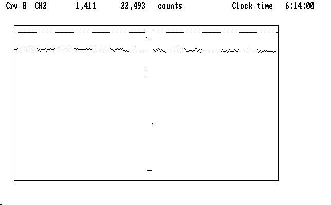
The marked sky in Ch1, at the top of the screen, tells us this is sky and not something else. Moving along, we encounter a region we might suspect to be a sky measurement in Ch2, but isn't:
| Fig. T10 |
Ch2 was interrupted for instrument alignment, and these points must be marked garbage. A real sky measurement appears on the right, certified by the presence of a sky measurement in Ch1. Of course, Ch1 can be interrupted without affecting Ch2 as well, so we must be on the lookout. When in doubt, check the counts, and compare with a "known" sky reading (e.g. one listed in the .log file for the run).
We'll mark the rest of Ch2 this way, then return Ch1 to its original size (Shift-PgUp) and we will see both curves, now fully marked and recompressed with 'x', as shown here:
| Fig. T11 |
Ctrl-Home brings the cursor back to the start of the light curve, so we can see the whole run on both channels. The Ins key puts the cursor back on Ch1.
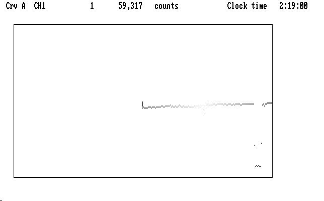
We are now finished with the tedious part of the reduction process. We'll do the rest of the required steps all at once with 'Ctrl-A', with the result shown below:
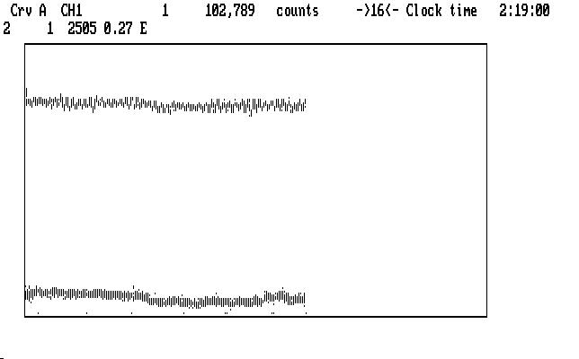
| Fig. T12 |
At this point the detector deadtime correction has been applied (key 'D'), the sky readings have been extracted ('T'), prepared by interpolation ('P'), and subtracted ('S') from each channel, and the extinction correction ('E') has been applied using the default values for the CTIO observatory, which Qed recognized on startup.
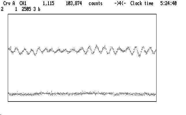
We're not quite finished. We must bridge over the places in the light curves where we took sky measurements, or removed bad data points. This can be done automatically when you write the data to disk, but you may want to see what this operation does to you, depending on the parameter you choose for the operation. The parameter is just the number of data points averaged together on each side of the bridge to anchor it, and it depends a bit on the chosen integration time (10 seconds in this case) and the pulsation periods in the star under study. We'll chose 5 points (50 seconds) and then bridge Ch1 by typing '5b'. The bridges start to blink, and you can expand the display ('x') and then run it past the cursor to see them in detail. Alt-LeftArrow will scroll the curve for you; '<-' or '->' will stop the scrolling.
We'll do the same thing with the Ch2 curve, but we must first put the cursor on it with the 'Ins' key -- lower case operations (like 'b') work on only one curve at a time. Channel 2 doesn't look great, and maybe we could do better with Ch1 as well -- there are several operations available, but we'll quit right here for now and write the data with 'F9'. The 'W' key does the same thing. We'll be able to come back to this point in the reduction very easily, if we later decide to touch things up. All of the operations we performed are encoded and recorded, and written to disk under the filename tol-0011.op1 along with the reduced data for each channel (tol-0011.1c and tol-0011.2c). Qed can replay the operations so you don't have to do them all over again, or any selected sequence of them, so you can change them later however you see fit.
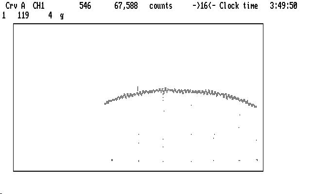
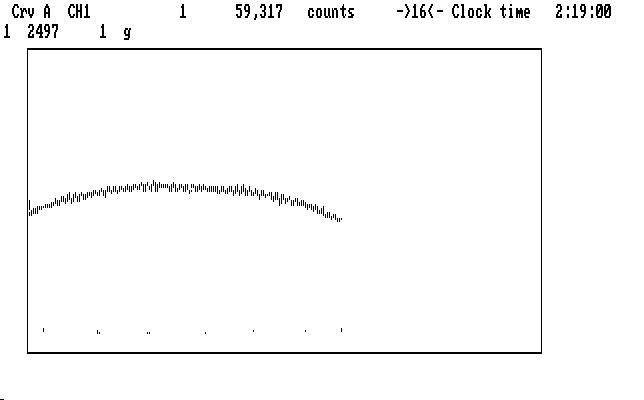
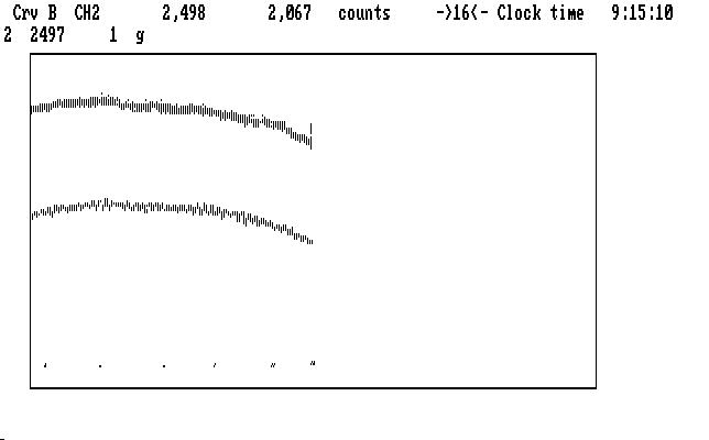
If we expand the X scale a bit, until we are only compressed by 4 instead of 16, scroll a bit, and magnify both curves by 2 (PgUp) we can see the pulsations we want to study in Crv A, shown below:
| Fig. T13 |
The bridged regions are blinking. As you can see, no damage has been done to the light curve by the bridging process.
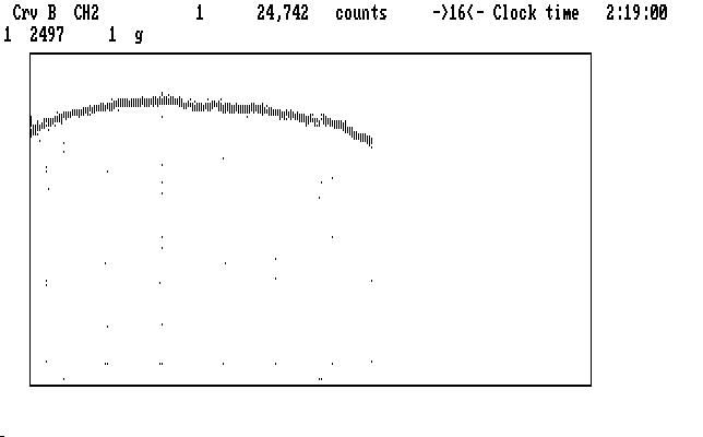
The oscialltions do not appear in Crv B. They'd better not! One of the reasons we reduce Ch2 as well as Ch1 is so we can be sure that instrumental cross-talk between channels is negligible. It usually is, but not always. We can use the Ch2 data in other ways, too, as we will see later.
We exit the Qed program with 'Ctrl-Shift-Esc'. Try to remember this keystroke combination; you can't stop Qed any other way, except by turning off the power to the computer. Stopping Qed in the middle of data reduction won't happen by accident if you don't kick the power cord.
You'll find three files in the working directory: tol-0011.1c (the reduced data for Ch1), tol-0011.2c (Ch2 reduced data) and tol-0011.op1, the list of recorded operations. Qed won't overwrite a file; it changes the endings of the filenames to avoid that. A second operations list on the same run will be named tol-0011.op2, the next will end with .op3, and so on. The ".1c" at the end means Ch1 with the 'c' (clear) filter; this gets changed to ".1ca" if a second data file, named ".1cb" gets written. If we ask Qed to split a run into two output files (by marking with '|' instead of 'g' somewhere) the output files are named this way.
If you want to save things "just in case" you can write the operations list at any time with 'Ctrl-W'. Some users like to save the .op list after they have finished marking, so they can start all over again if they mess things up, without having to do the marking all over again. If you start again, but have one or more .op files available, the command 'Ctrl-O' (that's Oh, not zero) will read in the latest one you wrote, which is usually what you want. If not, you can enter the number of an earlier one as a parameter, before the 'Ctrl-O' command, and Qed will read in that one instead. To read in tol-0011.op2 instead of tol-0011.op3, for example, type '2Ctrl-O'. If you want to find out which one Qed is using, type 'qo' and it will tell you.
Just so you have an overall picture of what we just did, here's a brief list showing the steps we go through to reduce a run:
One common cenvention is used everywhere: Upper case command letters refer to data in both channels, lower case only to the light curve the cursor is on ('Alt-S' is an honorary lower case command letter; through an ugly coincidence, both 'sky' and 'subtract' begin with the same letter).
Many additional operations are available, (e.g. dividing one light curve by the other, multiplying by a constant, adding or subtracting a constant, copying one data buffer to another, etc) and can be done at any time. The basic reduction sequence (D, T, P, S, E) is fixed, however, and Qed will insist that you do the operations in this order. The "macro-command" Ctrl-A, used in the example above, performs all the commands in this sequence on both light curves, using default values for any required parameters. Ctrl-N will do the next command in the sequence on both channels, whatever it is. Default values are remembered from previous reductions on runs using the same observatory and instrument, so once you build up the history file (qed.his), a single command can finish the job once the data are marked. You may prefer to do the steps one at a time, so you can see the result of each one, and you may want to set the verbosity threshold so Qed will tell you things it thinks you may want to know about after each step. You may also want to back up and change something -- perhaps the extinction coefficients -- the backup commands in Qed (Ctrl-B, Alt-B) let you back up any command operation so you can do it again. The marking operations are not affected by the backup process; they can only be changed with the unmarking operations.
| Previous Page | Contents | Next Page |